General Philosophy of the blog
When learning something new, I read chapters from books and papers related to the concept. Once I have some working knowledge on the subject, usually after 1-2 weeks of learning, I create a toy problem and simulate it in MATLAB with the aim of reproducing expected theoretical results. I love textbooks and papers that give worked out examples that I can readily try in MATLAB. Sometimes I find such examples on blogs or websites. After I have learnt the technical details and simulated a toy problem, I explain the concept to myself in layman terms. Forcing myself not to use technical jargon helps me push the learning to my long term memory. Here’s an example - I remember what convection heating is only because of the visual of green peas rising up in a pot of boiling water.
My goal for the technical section of the blog is to document some of these learnings in my not-so-technical style and also paste the toy problem code for others to try. I’ll also try to link the best books and papers that will give you all the technical information and jargon you need.
Random Processes and Random variables
If you went out to your balcony every hour between 8 AM to 8 PM and measured the wind velocity, you could put those readings on a plot of velocity (y-axis) vs time (x-axis) and you get one trace. If you did this for a week, and put all your traces on the same plot, you would have a bunch of messy lines on your plot. Now pick a time of the day, say 11 AM. Observe all the velocity readings you took at 11 AM on all days. They would appear randomly scattered. Now pick a day, say Monday. Observe the velocity readings you took for that complete day. These would also appear random.
We call wind velocity a random process 1. Each trace (corresponding to a day) is a realization of the random process. The value that the random process takes at a fixed time everyday (11 AM), is a random variable 1. If you take two random variables (say wind velocity at 10 AM and 11 AM everyday), then you can quantify how related the two seem by calculating the correlation of the two (referred as autocorrelation 1).
\[\Psi_{velocity}(10 AM, 11 AM) = E\{velocity_{10 AM} \times velocity_{11 AM}\}\]If the autocorrelation comes out to 0, this means nobody except Chuck Norris can tell you at 10 AM what the velocity will be at 11 AM. If the autocorrelation is non-zero, then at 10 AM you can assign a probability to the velocity at 11 AM and place bets with your friends. In general, between any two time instants $t_1$ and $t_2$, you get the autocorrelation function :
\[\Psi_{velocity}(t_1, t_2) = E\{velocity(t_1)\times velocity(t_2)\}\]For a stationary random process, the value of this autocorrelation only depends on the separation in the two time instants and not on the actual time instants 2. So if our wind velocity was a stationary process, you would have the same odds of winning money from your friend if you bet on the velocity an hour from whenever you speak to him. It wouldn’t matter when you agreed to start that hour.
Finally, the fourier transform (something that converts time domain signals to frequency domain signals) of the autocorrelation function (represented by $\bar{\psi}$)gives you the power spectral density of the random process. The power spectral density tells you the energy contained at each frequency of the random process.
White and coloured noise
Things are going to get a lot more technical from here…
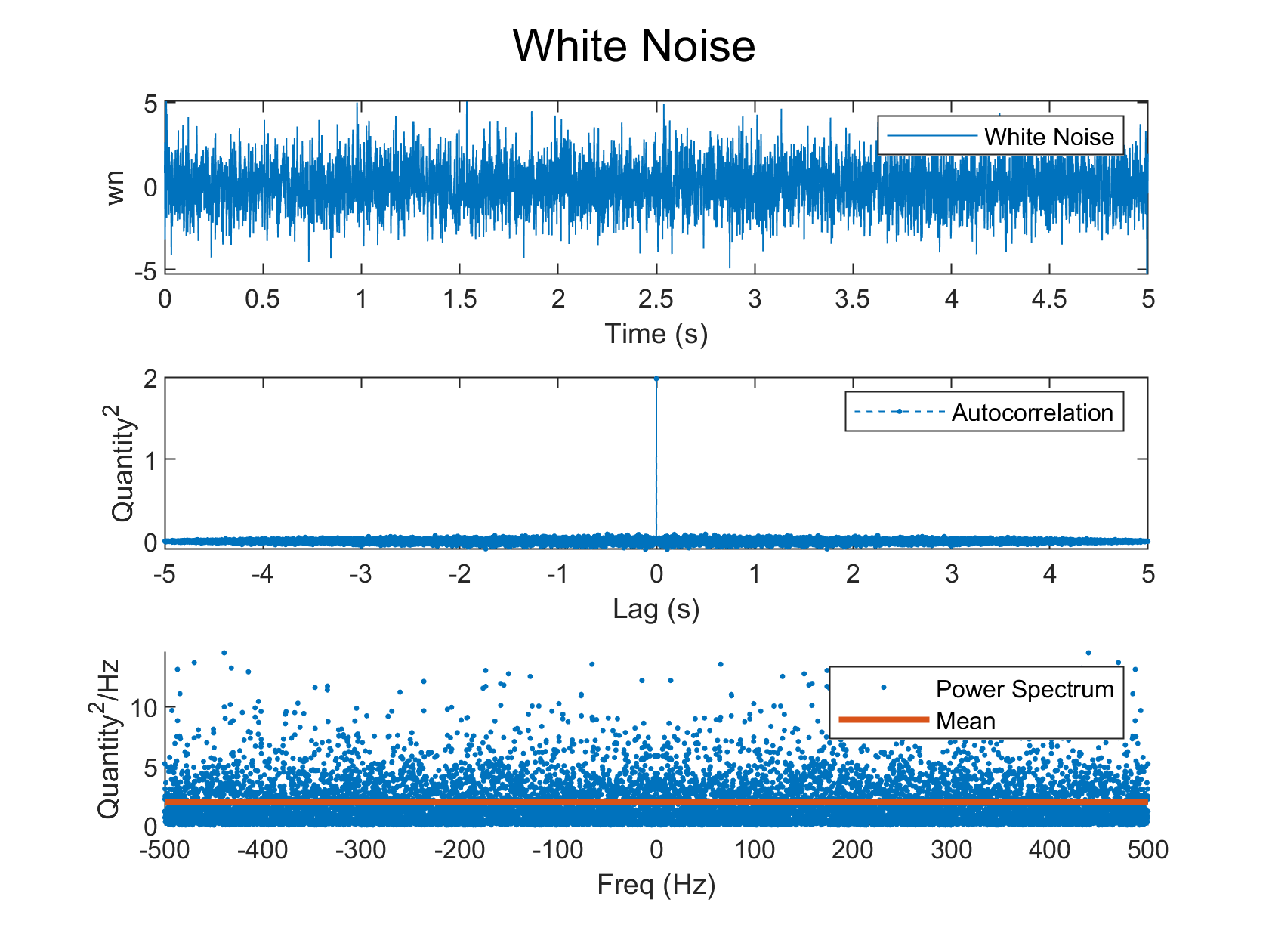
Gaussian white noise is a random process (lets call it $x$) that has an autocorrelation function that looks like the dirac delta.
\[\psi_{xx} = X_0\delta(\tau)\]$X_0$ is referred to as the strength of white noise. Additionally, the Gaussian nature of the process allows us to model each random variable in the process using the Gaussian probability distribution. Following the discussion from above, this means that as long as $\tau$, the difference in the time instants, is zero, there is no correlation between the two random variables. Intuitively, this also means that such a noise must have infinite energy. This is evident in its power spectral density - which is constant at all frequencies.
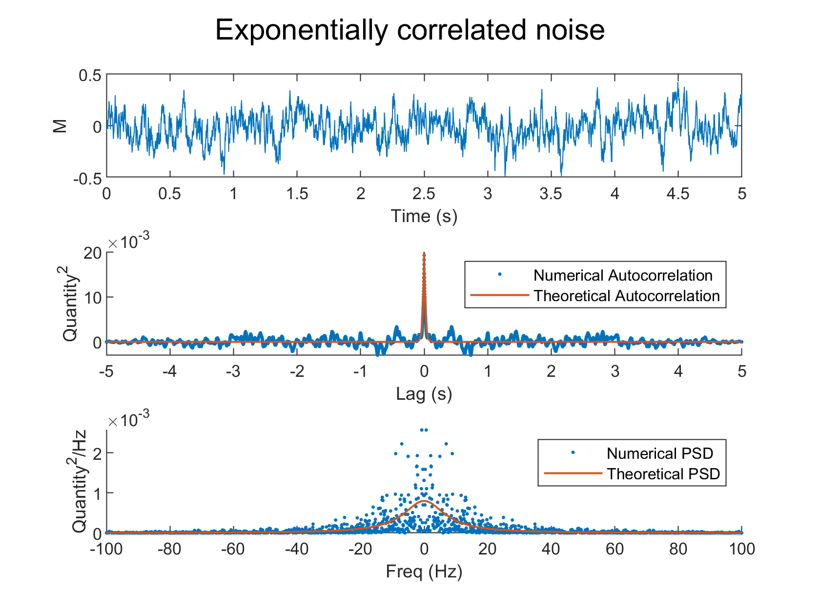
\[\bar\psi_{xx} = X_0\]Naturally, such a noise is fictitous for all meer mortals unless you’re Chuck Norris. A more realistic model of noise is Coloured Noise, which does not have infinite energy content. The simplest example of this is exponentially correlated noise. Its often easy to think of coloured noise as the output of some shaping filter 1 to which you fed in Gaussian white noise. That shaping filter can be modeled using Ordinary Differential Equations. If $M$ was the random process that we model using coloured noise, and $x$ was Gaussian white noise from before, then we would write :
\[\dot{M}(t) = -\frac{M(t)}{T} + x(t)\]$T$ is the correlation time constant that decides the bandwidth of this noise. That is, how wide in the frequency range does this noise have energy present ? The autocorrelation function and power spectral density of this noise are :
\[\begin{aligned} \psi_{xx} &= \sigma^2e^{-|\tau|/T}\\ \bar\psi_{xx}(\omega) &= \frac{2\sigma^2/T}{\omega^2 + (1/T)^2} \end{aligned}\]Simulating in MATLAB
To generate a realization of L samples from a Gaussian white noise process of strength $X_0$, you can use the MATLAB command sqrt(x0)randn(1,L). To generate a realization from the exponentially correlated process, you need to solve the differential equation. Although MATLAB has solvers such as ode45, we can’t use them for dynamic equations with Gaussian noise terms. First, we need to convert the ODE into Itô’s form3, which looks like this :
The last term ($d\beta$) is itself a Gaussian random variable (zero mean, and variance of $X_0dt$), and is interpretted as the difference in successive values of a Weiner Process 4. Here’s my interpretation - if you ask a drunk man to walk in a straight line, and trace his location on an X-Y graph, the trace will look like a Weiner Process. If you chop that trace into multiple steps, then each step is analogous to $d\beta$. The exact lemma that allows us to make the conversion from the ODE to Itô’s form is called Itô’s Lemma5.
With this setup, its very easy to use Euler integration in MATLAB to solve this differential equation in time. Here are the results from MATLAB that show, for Gaussian white noise and exponentially correlated noise, the following :
- A realization of the random process
- Autocorrelation : comparison of theoretically expected value and that obtained from the simulation
- Power Spectral Density : comparison of theoretically expected value and that obtained from the simulation


You can download the MATLAB script from here. You could also read more here.