I want to share a silly visual that I used to understand and remember the convolution integral that appears in the analytical solution of ordinary differential equations for linear systems.
Mass Spring Damper
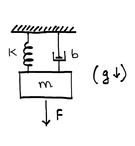
Linear Time Invariant (LTI) systems can be represented using ordinary differential equations. For example, look at the following mass spring damper (MSD) system (represented here by a beautiful free hand sketch).

The table below summarizes the meaning of each symbol, and the values I used for my simulation.
| Symbol | Meaning | Value | Units |
|---|---|---|---|
| m | Mass | 0.5 | kg |
| k | Spring constant | 10 | N/m |
| b | Damping coefficient | 1 | N/m/s |
| g | Acceleration due to gravity | 9.81 | m/s$^2$ |
| F | Input force | sin(2$\pi t$) | N |
If you are an engineer, you have seen this at least once before. If not, then many common applications use models such as this to represent system dynamics. For example, the wheels in your car can be approximated in some cases as a mass spring damper system (but inverted so that the base is excited instead of the mass). For a further reading, you can refer to this Wikipedia page. You can use Newton’s laws of motion to write the following differential equation :
\[m\ddot{x} + b\dot{x} + kx = F + mg\]Then you can convert this equation into the following state space form 1 :
\[\underbrace{\begin{bmatrix} \dot{v} \\ \dot{x} \end{bmatrix}}_{\dot{x}} = \underbrace{ \begin{bmatrix} -b/m & -k/m \\ 1 & 0 \end{bmatrix}}_{A} \begin{bmatrix} v \\ x \end{bmatrix} + \underbrace{ \begin{bmatrix} 1 & 1/m \\ 0 & 0 \end{bmatrix}}_{B} \underbrace{ \begin{bmatrix} g \\ F \end{bmatrix}}_{u}\]Velocities and forces are positive in the downward direction and $v$ is the velocity of the mass while $x$ is the spring compression. The response of an LTI system is a superposition of two components :
- Homogeneous response : MSD’s response only due to initial conditions. That means the behavior of the system when you release it from some initial position and ensure there is no external force you apply.
- Input response : MSD’s response due to inputs and zero initial conditions. This means we initialize the system from zero initial conditions but keep the input force.
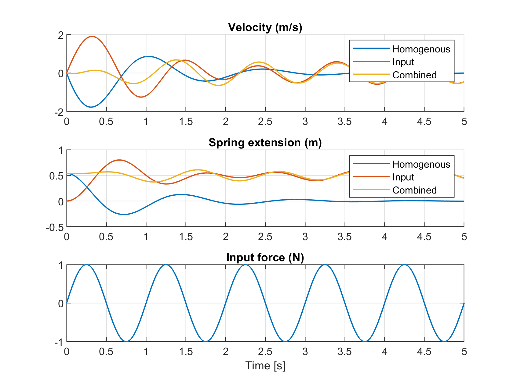
So for the MSD I sketched above, the following figure shows the homogeneous response, input response and the complete response of the system when released from an initial position and under a sinusoidal input force.

On careful observation, you will see that the total response is the sum of the other two responses. That figure was generated using a simulation of the linear system. However, being an LTI system, there is a neat way to get an analytical solution. Here is how that goes2 :
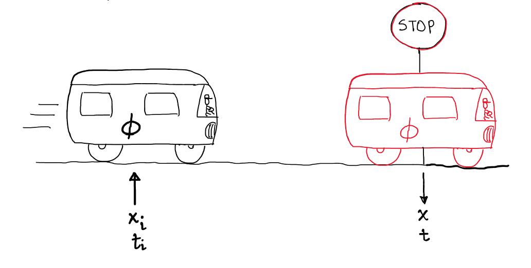
\[x(t) = \phi(t)x_0 + \int_0^t \phi(t,\tau)Bu(\tau)d\tau \tag{1}\]$\phi(t,t_i)$ is the state transition matrix and here is how understand it : its a bus that can take you from point $x_i$ at time $t_i$ to point $x$ at time $t$. In the equation above, I assumed that the initial time is $0$, and $\phi(t,0) = \phi(t)$.

Great sketch right ? The bus has a driver in there as well ! Anyways, the state transition matrix and the first term in the equation only takes care of the homogeneous response of the system. For LTI systems, you can calculate the state transition matrix using the matrix exponential, $\phi(t-t_i) = e^{A(t-t_i)}$. Things aren’t this straight forward for linear time-varying systems and you can refer to the book by D’Angelo3. The integral at the end of the equation is the topic of this post, and is called the convolution integral, or the matrix superposition integral. That is what gives us the response due to inputs. I know, TL;DR much ? Sorry.
Convolution Integral
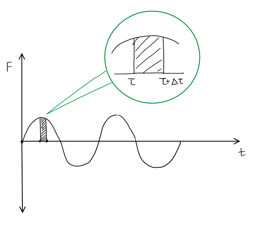
What follows is my silly way of understanding the convolution integral. For a more technically satisfying discussion, I recommend Section 3.3 from Gelb’s book (16th printing edition) 4. Lets view a sketch of the input signal (let’s stick to a single input for now), and chop it up into tiny pieces.

The green circle shows a zoomed in version of that small slice. If you continue chopping up the input signal this way until time $t$, with each slice of width $\Delta \tau$, you will get $\frac{t}{\Delta \tau}$ slices. As you start making $\Delta \tau$ smaller, those slices will start behaving like impulses. We have already established that the response of an LTI system can be seen as independent contributions from inputs and initial conditions. What’s great about this fact is that if the system is fed multiple inputs, the response from each input can be treated independently and the cumulative response is the superposition of all those responses.
Let’s think of the contribution of the complete input signal shown in the figure above as a superposition of the individual contributions from each of those tiny impulses. For now, let’s focus on the slice we had highlighted in the figure. That slice was an impulse occurring at time $\tau$ and lasting for $\Delta \tau$. You can approximate the slice as a rectangle, and calculate its value as the area under that rectangle.
\[Impulse = F(\tau)\Delta \tau\]You remember that bus ($\phi(t)$) from before that can take us from an initial time to a final time ? Well turns out if you load, at time $\tau$, an impulse input into the bus, then the contribution of that input to the final state at time $t$ is :
\[\Delta x_\tau = \phi(t,\tau) F(\tau)\Delta \tau\]Great, that’s one slice taken care of. How do we add the contributions from all the other impulse inputs ? Well you just add them up.
\[\Delta x_{total} = \sum\limits_0^t \phi(t,\tau) F(\tau)\Delta \tau\]As you start reducing $\Delta \tau$, the summation will change to an integration, and that’s how you get the convolution integral.
\[\Delta x_{total} = \int_0^t \phi(t,\tau) F(\tau)d\tau\]You can follow the same train of thought with multiple inputs, like we had in our MSD system ($B \ast u$) and you should be able to arrive at the convolution integral that appears at the end of equation 1 !
You can download the simulate file here and the model file that is called from the simulation file here.
References and Notes
-
Kailath, Thomas. Linear systems. Vol. 156. Englewood Cliffs, NJ: Prentice-Hall, 1980. ↩
-
Actually this equation is valid for Linear Time-Varying systems as well. ↩
-
d’Angelo, H. (1970). Linear time-varying systems: analysis and synthesis. ↩
-
Gelb, A. (Ed.). (1974). Applied optimal estimation. MIT press. ↩