Table of Contents
Overview
In Spring 2018, I took a course titled “Vehicle Systems Dynamics and Controls” (ME390) at UT Austin. The objective of the course was to teach concepts using first principles modeling and linear systems theory. One of the assignments, for example, was to pick a vehicle model of our choice, and try to make it follow a lane. As such, we were not expected to have the most accurate model or control systems, but rather we were expected to pick simple models, and try coming up with some lane following algorithms using first principles. Therefore, what you are going to see here is not the cutting edge, rather a toy problem that helped me understand how to pick a model, linearize it and apply state feedback. Later I applied the control law derived using the linear model, to the nonlinear model and simulated everything on MATLAB. We were also encouraged to animate the trajectory of the vehicle along with plotting the control errors. It was very fascinating to see the animation, and the idea of creating toy problems to understanding a concept and trying to visualize the outputs creatively has stayed with me to this day !
You can skip this article and just get the code on GitHub.
Here is how my final animation looked like.
Tricycle Kinematic Model
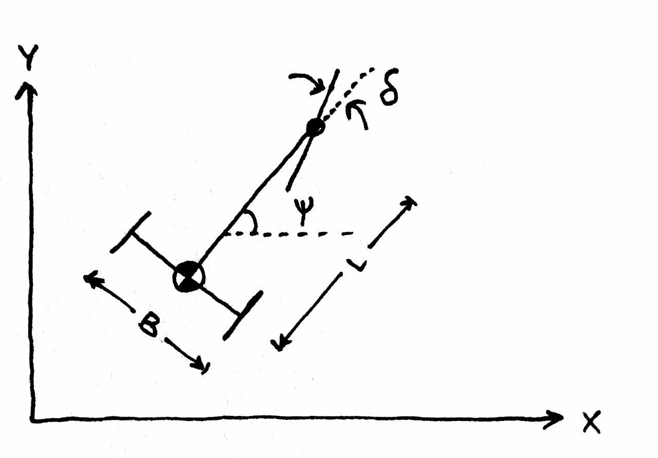
For the assignment, I picked a tricycle kinematic model. A sketch of the model is shown below.

Here, $B$ is the wheel base in meters, $L$ is the length of the chassis in meters, $\psi$ is the orientation in radians and $\delta$ the steering angle in radians. The following assumptions are made :
- The center of gravity of the tricycle is on the rear axle
- Use of small angle approximations is made when useful, i.e $\sin\delta \approx \delta, \cos\delta \approx 1$
- The vehicle is always moving with a constant forward velocity of $v$ meters per second
The dynamic equations can be written as :
\[\begin{aligned} \dot{x} &= v\cos\psi \\ \dot{y} &= v\sin\psi \\ \dot{\psi} &= \frac{v}{L} \tan\delta \end{aligned}\]If we apply small angle approximation, then the overall model in state space form is as follows.
\[\begin{bmatrix} \dot{x} \\ \dot{y} \\ \dot{\psi} \end{bmatrix} = \begin{bmatrix} 0 & 0 & 0 \\ 0 & 0 & v \\ 0 & 0 & 0 \end{bmatrix} \begin{bmatrix} x \\ y \\ \psi \end{bmatrix} + \begin{bmatrix} 0 \\ 0 \\ v/L \end{bmatrix}\delta + \begin{bmatrix} 1 \\ 0 \\ 0 \end{bmatrix}v\]Treating $\delta$ as our only control variable, we realize that this system is not fully controllable. However, we realize that the state $x$ is dependent, because it is fully determined by the known forward velocity $v$ and the state $\psi$. If we remove it from the system, the remaining 2x2 system is fully controllable. The new state space representation is as follows.
\[\begin{bmatrix} \dot{y} \\ \dot{\psi} \end{bmatrix} = \begin{bmatrix} 0 & v \\ 0 & 0 \end{bmatrix} \begin{bmatrix} y \\ \psi \end{bmatrix} + \begin{bmatrix} 0 \\ v/L \end{bmatrix}\delta\]The new system is fully controllable.
Rate of change of orientation
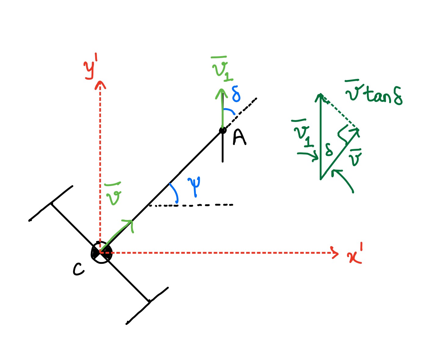
I had to scratch my head a little at the last of those equations so I wanted to document my understanding here. You can skip this part. Let’s look at the velocities of the center of gravity of the vehicle, and the point where the front wheel would be attached to the vehicle.

Imagine that we are observing the vehicle from an intermediate frame $x’y’$ that is attached to the center of gravity. This frame translates along with the vehicle, but does not rotate relative to the absolute reference frame. From this relative frame, we can find the velocity of point $A$ that is perpendicular to line segment $CA$. The figure showing the velocity vectors makes the trigonometry apparent so that we can find that velocity to be $v\tan\delta$. There after, we know that the angular velocity is $\dot{\psi}_{x’y’} = \frac{v}{L}\tan\delta$. Since the segment $CA$ can be treated as a rigid segment, it’s total angular velocity will be that observed from the relative frame of reference plus the angular velocity of that frame. In our case, $x’y’$ does not rotate, therefore $\dot{\psi} = 0 + \frac{v}{L}\tan\delta = \frac{v}{L}\tan\delta$.
Control Law
I chose to use state feedback, which for the 2x2 reduced order system would give us a control law of the form:
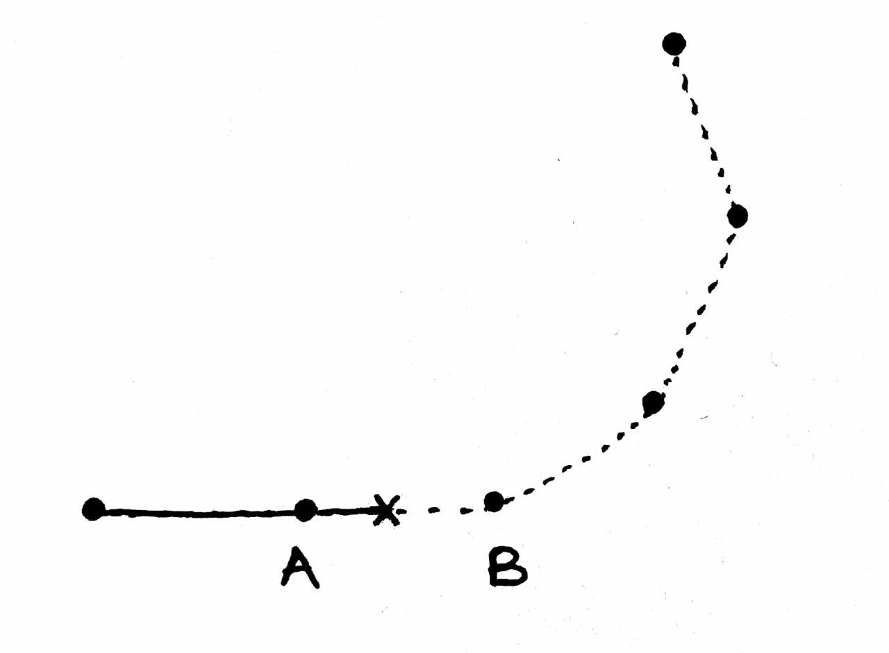
\[\delta = -k_1(y - y_{des}) - k_2(\psi - \psi_{des})\]Where $y_{des}, \psi_{des}$ represent the desired y location and orientation of the vehicle. This is another place I had to scratch my head. How would we know the desired setpoints ? I made the assumption that the U turn is made of linear segments, and that we know the coordinates of the entire track. Since the vehicle traverses with constant forward velocity $v$, we can calculate where on the track it must be, and represent this point with a “desired position” pin.

At every time step, we have two “goals”, that we call points $A$ and $B$. These represent the linear section of the track which the vehicle must traverse on. The pin marked with an x in the figure above represents the desired position pin (call it $z_{des}$) at time “$t$”, and the solid line shows the path already covered. The control task for the vehicle is to be as close to this pin, and cover the linear segment from $A$ to $B$. Once we are done with this segment, the algorithm updates the points $A$ and $B$ for the next set of iterations. This can be done using the following update equation.
\[\boldsymbol{z}_{des} = \boldsymbol{A} + vt\frac{\boldsymbol{B} - \boldsymbol{A}}{|\boldsymbol{B} - \boldsymbol{A}|}\]Where $|.|$ represents the norm of the vector. This parametric equation can update the desired position pin every time step. In my code, the following lines do the job of always updating these goal points.
if norm(des_pos - A) >= base_norm
  % Update A and B
  track_index = track_index + 1;
  t_marker= t-(norm(des_pos - B)/v);
  A = [xtrack(track_index); ytrack(track_index)];
  B = [xtrack(track_index + 1); ytrack(track_index + 1)];
  base_norm = norm(B - A);
end
The desired orientation can be calculated as follows :
\[\psi_{des} = \tan^{-1} \left( \frac{(B - A).\hat{j}}{(B - A).\hat{i}}\right)\]I used MATLAB’s place command to get the gains based on desired pole locations.
MATLAB Code
That’s about it ! I coded everything up in MATLAB, and added some functions I found on the internet for drawing a cartoon of the tricycle and animating it. Although the control law is derived with a linearized version of the model, the nonlinear plant model (the very first state space representation) was simulated and fed the $\delta$ dictated by the controller. The code can be found on GitHub. Once again, there is nothing fancy in terms of the model or control algorithms, but the goal of the toy problem was to get a basic understanding of linearization and state feedback. Besides the regular plots, animating the simulation added another layer of excitement and joy and that made the class all the more interesting 😁